Use SUMIF as VLOOKUP
This tutorial shows how to use the the SUMIF function as a VLOOKUP function allowing for greater flexibility


|
GENERIC FORMULA
=SUMIF(range1,criteria1,INDEX(sum_range,,MATCH(criteria2,range2,0)))
ARGUMENTS GENERIC FORMULA
=SUMIF(range1,criteria1,INDEX(sum_range,,MATCH(criteria2,range2,0)))
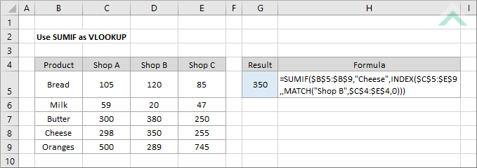
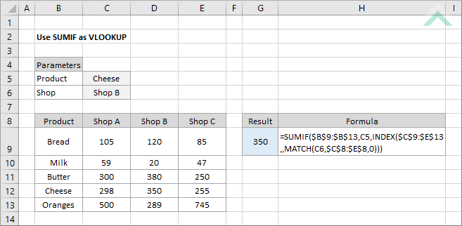
ARGUMENTS EXPLANATION This tutorial shows how to use the the SUMIF function as a VLOOKUP function. Using the SUMIF, INDEX and MATCH functions you gain greater flexibility and functionality to sum values with associated criteria. By using the VLOOKUP function you can only return the first value associated with a single criteria, whilst using this formula you can return a sum of numbers associated with multiple criteria.
Click on either the Hard Coded or Cell Reference button to view the formula that has the criteria 1 and 2 directly entered into the formula or referenced to a specific cell. |
| Related Topic | Description | Related Topic and Description |
|---|---|---|
| Two dimensional lookup with VLOOKUP and MATCH | How to apply a two dimensional lookup with VLOOKUP and MATCH functions | |
| Two dimensional lookup with INDEX and MATCH | How to apply a two dimensional lookup with INDEX and MATCH functions |
| Related Functions | Description | Related Functions and Description |
|---|---|---|
| SUMIF Function | The Excel SUMIF function returns the sum of all numbers in a specified range based on a single criteria | |
| MATCH Function | The Excel MATCH function searches for a specified value in a range and returns its position relative to the range | |
| INDEX Function | The Excel INDEX function returns a value that is referenced from a specified range |
