Two dimensional lookup with VLOOKUP and MATCH

This tutorial shows how to apply a two dimensional lookup using a combination of the Excel VLOOKUP and MATCH functions

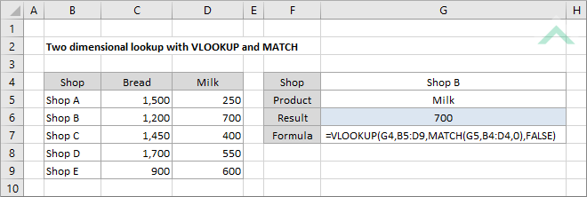
Example: Two dimensional lookup with VLOOKUP and MATCH

METHOD 1. Two dimensional lookup with VLOOKUP and MATCH

EXCEL

=VLOOKUP(G4,B6:D9,MATCH(G5,B4:D4,0),FALSE)

The formula uses the Excel VLOOKUP and MATCH functions to return the value that is associated with Shop B and Milk. The formula initially looks up the row that contains Shop B in range (B6:B9), which is achieved with a VLOOKUP function. The VLOOKUP function then requires the relevant column number of the selected range, that is associated with Milk. This is achieved with a MATCH function which searches for the specified value, in this example it's Milk, and returns its position relative to the range.

METHOD 1. Two dimensional lookup with VLOOKUP and MATCH using VBA

VBA

Sub Two_dimensional_lookup_with_VLOOKUP_and_MATCH()

'declare a variable
Dim ws As Worksheet

Set ws = Worksheets("Analysis")

'apply the two dimensional lookup formula using VLOOKUP and MATCH
ws.Range("G6").Value = WorksheetFunction.VLookup(ws.Range("G4"), ws.Range("B6:D9"), WorksheetFunction.Match(ws.Range("G5"), ws.Range("B4:D4"), 0), False)

End Sub

OBJECTS
Worksheets: The Worksheets object represents all of the worksheets in a workbook, excluding chart sheets.
Range: The Range object is a representation of a single cell or a range of cells in a worksheet.

PREREQUISITES
Worksheet Name: Have a worksheet named Analysis.
VLookup Range: If using the exact VBA code ensure that the range ("C5:D9") captures the data that you want to return and range ("B5:B9") captures one of the values that you are looking up.
Match Range: If using the exact VBA code ensure that the range ("B4:D4") captures the other value that you are looking up.

ADJUSTABLE PARAMETERS
Output Range: Select the output range by changing the cell reference ("G6") in the VBA code to any cell in the worksheet, that doesn't conflict with the formula.
VLookup Range: Select the data range and the range that captures one of the values that you are looking up by changing range reference ("B6:D9") in the VBA code to any range in the worksheet, that doesn't conflict with the formula.
Match Range: Select the range that captures the other value by changing range reference ("B4:D4") in the VBA code to any range in the worksheet, that doesn't conflict with the formula.

Explanation about how to apply a two dimensional lookup using a combination of the Excel VLOOKUP and MATCH functions

EXPLANATION

EXPLANATION
To apply a two dimensional lookup we can use a combination of the Excel VLOOKUP and MATCH functions.

FORMULAS
=VLOOKUP(lookup_value_1,table,MATCH(lookup_value_2,range,0),FALSE)

ARGUMENTS
lookup_value_1: The value you want to lookup in the first column from the selected range (table).
lookup_value_2: The value you want to lookup in the first row from the selected range (table)
table: A table of data from which to lookup the value. The first column of this table will also capture lookup_value_1.
range: A range that captures the lookup_value_2.